Working with a Dataset
Loading a dataset.
The quickest way to get started with ApertureDB is to load a simple dataset containing some images and metadata but without a complex schema. Most Kaggle datasets will load into ApertureDB with minimal modifications (for a more complex example, see our celebrity faces loader).
There are multiple ways to load data into ApertureDB, as discussed in Ingest Data And Metadata, but with a pre-existing dataset, the quickest way is to ingest using a CSV file.
For following along with this document, we've produced a subset of the Stanford Cars Dataset to create a small CSV file as a sample of what a CSV file might look like (more examples here). You can use your own dataset if you want, and we will make out things you might need to change.
Tools Needed
To load a dataset, you will need
- ApertureDB credentials and instance (you can use the docker instance for a simple server)
- A system with Python 3+ installed
- ApertureDB Python package ( installed with
pip install aperturedb) - A dataset to load and query
- Jupyter notebook or just command-line execution of Python samples
Setup
On your system with the aperturedb package installed, first you will need to download your dataset. The sample used in this document is the miniature Standford Cars Dataset. The archive contains images and a csv.
wget https://aperturedata-public.s3.us-west-2.amazonaws.com/sample_images/demo-slim-stanford-car-dataset.zip
Next, uncompress the dataset:
unzip demo-slim-stanford-car-dataset.zip
cd slim-stanford-car-dataset
Create CSV Input
Now we need to make a CSV file that will tell ApertureDB how to load our data.
In this guide we will assume that we are uploading images and associated properties with each image. The columns in the CSV file will be of 3 types
- filename - points to the image to load - always the first column, called 'filename', 'url', 's3_url' or 'gs_url'.
- constraint - input to limit which files are uploaded (like a primary key check in relational db).
- properties - anything else without 'constraint_' as a prefix is basically image metadata
Many datasets will come with a CSV file which has properties, but some many not have any. To make a minimal CSV file in that case you would run something like
echo "filename" > dataset.csv && find -iname \*.jpg >> cars.csv
which would make a CSV file with 1 column containing the names of the files to load.
The Stanford dataset we have provided contains a CSV file called cars.csv.
Now that we have a CSV file, we need to ensure it meets our needs.
In a Jupyter cell or input.py, you can add the following and run the cell or try
python input.py:
import pandas as pd
df = pd.read_csv('cars.csv')
print(df)
Output:
    filename        make    model  year   color    style   angle
0  00001.jpg        audi       a7  2012   white    sedan  angled
1  00002.jpg       acura       tl  2014   black    sedan  angled
2  00003.jpg       dodge      ram  2009     red    truck  angled
3  00004.jpg     hyundai   sonata  2015     red    sedan    rear
4  00005.jpg        ford    f-350  2016   white    truck  angled
5  00006.jpg       izuzu   tracer  2007     red  compact  angled
6  00007.jpg       dodge  journey  2015    blue      suv  angled
7  00008.jpg       dodge  charger  2017     red   sports  rangle
8  00009.jpg  mitsubishi   galant  2012  silver    sedan   angle
9  00010.jpg   chevrolet  equinox  2017  silver      suv    side
Customize Your CSV
We will modify some columns because sometimes you may not care about data, or possibly some columns are partially empty or otherwise unhelpful. ApertureDB loaders also expect certain columns in the CSV files.
df.drop( ["year","style"], axis=1, inplace=True)
Another common issue is that sometimes the file information might not be relative. In our sample data, this is the case.
old_filename = df['filename']
df['filename'] = [ 'cars/cars_train/cars_train/' + name for name in old_filename ]
This will ensure the filename is relative to the csv file - a requirement for loading in ApertureDB when using the CSV loaders.
Now we'll show creating a new column with existing data. Say you want to make an id column that doesn't have the leading zeros.
from pathlib import Path
df['id'] = [ int( Path(file).name.split(".")[0]) for file in old_filename ]
This can be very useful if some of the data had different file types, such as .png - then your queries can just search for id == 20 and not have to know if it is 00020.jpg or 00020.png.
Finally, we'll add a unique identifier constraint so if you re-run the load it won't try to duplicate the data, then show what this looks like, and output it to a CSV file.
df['constraint_id'] = df['id']
print(df)
df.to_csv('modified_cars.csv',index=False)
Output
                               filename        make    model   color   angle  id  constraint_id
0  cars/cars_train/cars_train/00001.jpg        audi       a7   white  angled   1              1
1  cars/cars_train/cars_train/00002.jpg       acura       tl   black  angled   2              2
2  cars/cars_train/cars_train/00003.jpg       dodge      ram     red  angled   3              3
3  cars/cars_train/cars_train/00004.jpg     hyundai   sonata     red    rear   4              4
4  cars/cars_train/cars_train/00005.jpg        ford    f-350   white  angled   5              5
5  cars/cars_train/cars_train/00006.jpg       izuzu   tracer     red  angled   6              6
6  cars/cars_train/cars_train/00007.jpg       dodge  journey    blue  angled   7              7
7  cars/cars_train/cars_train/00008.jpg       dodge  charger     red  rangle   8              8
8  cars/cars_train/cars_train/00009.jpg  mitsubishi   galant  silver   angle   9              9
9  cars/cars_train/cars_train/00010.jpg   chevrolet  equinox  silver    side  10             10
A column that is used as constraint gets indexed automatically. If you are loading with any other method, check if you have created an index. Otherwise the load can be slow. It is, of course, fastest without any constraints.
Load the CSV File
First we'll define a function to do the loading either in a Jupyter cell
or in a load.py script.
from aperturedb.Connector import Connector
from aperturedb.ImageDataCSV import ImageDataCSV
from aperturedb.ParallelLoader import ParallelLoader
def load_image_and_metadata(dbconn:Connector, path_to_csv:Path):
    image_csv = ImageDataCSV(str(path_to_csv))
    loader = ParallelLoader(dbconn)
    loader.ingest(image_csv)
As you can see, this part is really easy, because all the difficult part has been done!
Now all we need to do is run it. We'll assume you've already configured your connection in the environment.
Load Method 1 :
from aperturedb import Utils
conn = Utils.create_connector()
load_image_and_metadata( conn, Path('modified_cars.csv'))
Load Method 2 : You can also use the adb command line to load the data:
adb ingest from-csv modified_cars.csv --ingest-type IMAGE
Checkout transformers like CLIP embedding generation when loading images with the adb command line.
This is a good time to use the web UI and navigate the cars in your database.
Query Your Data
Now we can check to see if your data loaded correctly. You can copy
this and run in a notebook cell or create a query.py file:
from aperturedb import Utils
conn = Utils.create_connector()

count_query=[{
   "FindImage": {
        "blobs":False,
        "results": {
            "count":True
        }
   }
}]
result,blobs = conn.query(count_query)
print(conn.get_last_response_str()) # prints result with JSON formatting
Output
[
    {
        'FindImage': {
            'count': 10,
            'returned': 0,
            'status': 0
        }
    }
]
Filter Using Metadata
Now, with the existing connection, we will choose only a subset to download / display - the red cars.
count_query=[{
   "FindImage": {
        "blobs": True,
        "constraints": {
            "color": ["==","red"]
        },
        "results": {
            "count": True
        }
   }
}]
red_car_result,red_car_blobs = conn.query(count_query)
print(conn.get_last_response_str())
Output
[
    {
        'FindImage': {
            'blobs_start': 0,
            'count': 4,
            'returned': 4,
            'status': 0
        }
    }
]
Visualize Data
The example below, requires you to run it in a jupyter notebook. A simple visualization of the data as a grid display:
This requires 3 packages inside the notebook: aperturedb, PILLOW and ipyplot (all can be installed using pip).
If you have never installed packages inside a notebook, you can do the following:
!pip install aperturedb Pillow ipyplot
First we define a function to save images to disk after resizing.
from pathlib import Path
from io import BytesIO
import PIL
def save_images(input_blobs, save_path:Path, name_func):
    images = []
    labels = []
    for i,img in enumerate(input_blobs):
        with BytesIO(img) as img_bytes:
            pil_img = PIL.Image.open( img_bytes)
            dim_max = max(pil_img.height, pil_img.width)
            scale = dim_max/256.0
            w = int( pil_img.width / scale )
            h = int( pil_img.height / scale )
            pil_img_resized = pil_img.resize( (w,h) )
            file_name = "{0}.jpg".format( name_func(i) )
            path = save_path.joinpath( file_name )
            print(f"dim_max: {dim_max}, scale: {scale}, w: {w}, h: {h}, file_name: {file_name}, path: {path}")
            images.append(pil_img_resized)
            labels.append(file_name)
    return images,labels
then we display them
from ipyplot import plot_images

def make_car_name(blob_index):
    return f"car-{blob_index}"
images,labels = save_images( red_car_blobs, Path("./data"), make_car_name )
plot_images(images,labels,img_width=150)
Quick glance through the WebUI
You can see your images visually if you use the docker-compose for web-ui in the setup instructions.
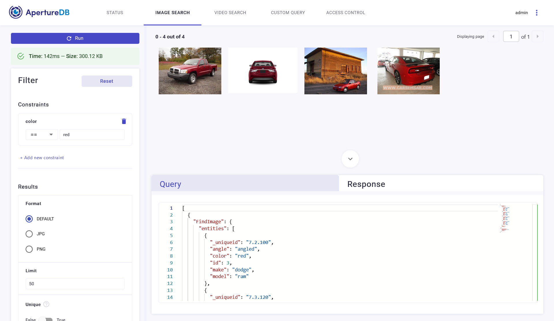
Red cars on the ApertureDB UI
Next Steps
Now that you have seen how easy it is to load and retrieve a dataset with images, you can find your own dataset, create or manipulate a CSV file describing them and load all of it into ApertureDB. You can also create your own example application following the steps outlined here.
Let us know if this helped!